






This document describes the methodology Oenra Labs uses to evaluate frontier wines against one another within a defined category. A study recruits a panel of independent domain experts, presents each evaluator with the pours from several producers on a shared set of flights under blinded and randomized conditions, and collects three classes of response: forced-choice rankings, scalar quality ratings on named rubric dimensions, and free-text rationale. Where the tasting programme spans more than one stage of service, the same instrument is administered at each stage so that performance can be tracked across the tasting window.
The resulting data is analyzed with a combination of pairwise tournament statistics, Bradley-Terry strength estimation, scalar rating summaries, structured qualitative coding of free-text responses, and a panel of inter-rater reliability diagnostics. Rubric details, panel size, wine count, phase taxonomy, and flight structure vary by study. The methodology described below is constant. The same instrument also feeds the cross-study leaderboard on the research hub: section 1 describes how the per-study results are pooled into a single ranking, and sections 2 through 7 describe the study methodology that produces them.
1. The cross-study leaderboard
The Best Performing Wines leaderboard on the research hub is not a single study. It is a single strength score for each red bottling, pooled across all of the included studies, that powers the Reds tab. This section describes how that score is fit and what it can and cannot tell you.
1.1 Hierarchical Bradley-Terry with partial pooling
This leaderboard estimates a single strength score for each red bottling by pooling pairwise preferences across all of the included studies, while allowing each study to influence the wine in its own way.
Each wine gets two pieces of information. The first is a global strength that reflects how the wine performs across every study it appeared in. The second is a per-study adjustment that captures how the same wine does on one specific flight relative to its global average. The final score on the leaderboard is the global strength.
The amount of pooling between these two pieces is learned from the data, not chosen by hand. We hold out one fifth of the (tournament, flight) units, refit the model on the rest at a range of pooling settings, and pick the settings that best predict the held out comparisons. To keep the search well behaved with only thirteen wines, we add a weakly informative half-Normal prior on the global spread. The prior allows the data to pull the spread up if the evidence supports it, but keeps it from collapsing to an unrealistically small value when there is little to estimate it from.
Once the pooling settings are fixed, the model is refit on the full dataset. Scores are converted to an Elo-style scale anchored around 1000 so higher numbers mean stronger preferences across studies. Uncertainty is estimated with a cluster bootstrap. Each bootstrap iteration resamples whole (tournament, flight) units rather than individual head to head comparisons, which preserves the dependency between comparisons that come from the same evaluator looking at the same flight.
The effect of partial pooling shows up most clearly for wines with thin coverage. A wine that only appeared in one or two studies has very little independent information in the data, so its global score gets pulled toward the field average. A bottling with broad coverage has plenty of evidence on its own, so its score is largely driven by its own win record. This is the property that makes the leaderboard more honest as a cross study signal.
1.2 Limitations
This is a cross study preference signal, not a controlled benchmark. It is the strongest summary we can produce from the data we have, but it inherits a number of issues that no amount of statistical machinery can fully fix.
The included studies are not comparable in the way that a controlled experiment would require. They vary by study type, flight set, evaluator pool, and the slate of wines that participated. Two wines that never met in any study are still ranked relative to each other through their shared opponents, which is a useful but indirect comparison.
Coverage is uneven. Some wines appeared in many studies and some appeared in only two. The hierarchical model handles this by shrinking low coverage wines toward the average, but it cannot create evidence that does not exist. Rankings for low coverage bottlings should be read as provisional.
The bootstrap intervals capture variation across the tournaments that were actually run. They do not capture the variation that would come from running a different set of studies, choosing a different flight set, or using a different evaluator pool. The true uncertainty is wider than the intervals shown.
Bradley-Terry assumes a single latent ranking exists. Preferences over wine in the glass often violate this in subtle ways. The same wine might win consistently against one type of opponent and lose consistently to another for reasons that do not fit on a single line. The leaderboard summarizes the average tendency and hides this kind of structure.
Evaluators are treated as interchangeable. There is no per evaluator effect, no weighting by evaluator quality, and no accounting for the possibility that some evaluators have systematic preferences for certain wines or styles.
The Elo scale is anchored to the mean of the included wines. Adding or removing a bottling from the dataset shifts the absolute numbers even when the underlying preferences are unchanged. Only the ranks and the gaps between wines are stable across versions of the leaderboard.
The hierarchical model captures task specific behavior in the per-study adjustments but uses only the global strength for the final ranking. This is the right design for a cross study summary, but it does mean that a wine with strong task specific strengths can look weaker on the leaderboard than it would in a single domain study.
The leaderboard should be read as a directional signal. Where confidence intervals overlap, the ranks should be treated as a tie. It is most informative for bottlings with broad coverage and many completed tournaments, and least informative for bottlings that appeared in only one or two studies.
2. Research questions
Each Oenra Labs study is designed to answer four questions about a defined wine category:
- Which wine is preferred overall, and by what margin.
- Where each wine wins or loses, decomposed across rubric dimensions, flight types, and (where applicable) service stage.
- Why evaluators preferred one pour over another, in their own words.
- How much weight the panel's conclusions deserve, given the agreement among evaluators.
The first two questions are addressed quantitatively. The third is addressed by structured analysis of free-text responses. The fourth is addressed by a battery of inter-rater reliability diagnostics. Quantitative and qualitative findings are reported jointly so that effect sizes are paired with mechanistic explanations.
3. Evaluation environment
Studies are conducted inside an internal evaluation application maintained by Oenra Labs. Evaluators authenticate, receive an assigned set of flights (referred to as tournaments), and complete each tournament as a self-contained task.
Within a tournament, the evaluator is shown the pours from every participating producer for a single flight. Pours are presented in randomized order and labelled with neutral identifiers (Wine A, Wine B, and so on), so the evaluator cannot infer which pour came from which producer. Where applicable, a reference sample (control bottle, house standard) is shown alongside the pours.
The evaluator completes the ranking, the scalar ratings, and the rationale text before the next tournament is revealed. All responses are timestamped and recorded at the grain of (evaluator, flight, wine).
For studies that span more than one stage of service in the glass, the same evaluator typically reviews pours from each producer at each stage of the tasting within the same session, with stages presented in their natural service order. Common service taxonomies include first pour, decanting, and the finish for still-wine tastings, but the number and naming of phases varies by category.
4. Instrument: question types
A study uses a combination of three question formats. Most studies use all three. The exact rubric is calibrated to the wine category under evaluation.
4.1 Forced-choice rankings
The evaluator is shown the pours from N wines for a single flight and asked to place them in rank order, from best to worst, against a stated criterion. Internally, an N-way ranking is decomposed into N choose 2 pairwise comparisons for downstream analysis. Rankings capture relative judgment, which prior work in psychophysics and preference modeling has shown to be substantially more reliable than absolute rating when the panel is heterogeneous (see §6).
In many studies the evaluator is also asked, after submitting a ranking, to indicate their confidence in that ranking on an ordered scale (for example, low, medium, high). Confidence responses are reported as a separate distribution and used to weight or filter rankings during sensitivity analysis.
4.2 Scalar ratings
For each wine poured, the evaluator assigns a 1-to-5 score on each of several named rubric dimensions. Rubric dimensions are chosen so that they are conceptually orthogonal and so that, in aggregate, they decompose the construct of quality for the category under study.
A study's rubric typically contains between three and seven scalar dimensions. Studies of young red wine may rate tannin structure, varietal typicity, and length of finish. Studies of sparkling wine may rate the mousse, colour and clarity, and fine balance. Studies of aged wine may rate tertiary aroma, oxidative drift, and fruit persistence. The specific rubric is set during study design and held constant across all evaluators and flights within a study.
Scalar ratings make it possible to characterize absolute quality on each dimension, not only relative quality. They are the noisiest signal collected and therefore require explicit reliability diagnostics (see §6).
4.3 Free-text rationale
After ranking and rating, the evaluator is asked to justify their judgment in writing. Common question formats include:
- Strengths and weaknesses questions. What did each wine do well. What did it miss.
- Per-comparison questions. Why did you rank wine X above wine Y.
- Failure-mode questions. Describe the most jarring defect in any pour.
- Phase-transition questions (for multi-phase studies). What changed between this stage and the previous one, and was the change positive or negative.
Free-text responses are the input to the qualitative analysis described in §5.7 and §5.8.
4.4 Flight construction
Flights are the experimental stimuli. The credibility of every downstream finding depends on the flights being representative of real-world drinking, broad enough in scope to surface wine differences, and not selected in a way that favors any one wine. Oenra Labs builds the flight set for a study in four steps.
Sourcing. Flights are drawn from real buyer briefs, partner-supplied line-ups, and synthesized analogues that mirror common purchasing tasks in the target category. Flight briefs are rewritten where necessary to remove identifying client information but are otherwise kept close to their source form. Wholesale invention of flights is avoided; the goal is for an evaluator reading the brief to recognize a line-up they could plausibly pour at work.
Taxonomy and balance. Flights are categorized along the dimensions the study intends to dissect. For a red-wine benchmark this might be vessel and closure (natural cork, screwcap, composite) and price band (entry, mid-market, premium, icon tier). For a white-wine benchmark it might be region, oak regime, and residual sugar level. The flight set is balanced across categories so that no single segment dominates the aggregate result and per-segment analyses (§5.5) have sufficient observations.
Validation. Every flight is reviewed before the study runs. The review checks that the flight is unambiguous, that it does not contain a wine that every taster can identify in a trivially obvious way, and that the requested comparison falls within the rated rubric. Flights that are degenerate (for example, flights where all participating wines present as sensorially identical) are removed during this pre-pour review or, if missed, excluded during data cleaning and reported as such in the study's QA section.
Volume. A typical study uses between fifteen and forty flights, depending on the number of bottlings in the comparison, the size of the panel, and the cost of each individual judgment. Flights are assigned to evaluators on a partially overlapping schedule so that every flight receives multiple independent rankings and so that inter-rater reliability (see §6) can be computed on a per-flight basis.
5. Analysis
An Oenra Labs analysis notebook produces the following outputs for every study. Within a single-phase study, each block is computed once. Within a multi-phase study, each block is computed separately for each phase, and §5.10 cross-phase comparisons are added on top.
5.1 Pairwise win-rate matrix
For every ordered pair of wines (A, B), the proportion of evaluator-flight observations on which A was ranked above B is computed and rendered as a wine-by-wine heatmap. The pairwise matrix is the rawest possible expression of the preference data, prior to any modeling assumptions. It exposes non-transitive patterns (where A beats B, B beats C, and C beats A) that would be hidden in a single-number summary, and provides the ground truth against which the Bradley-Terry estimates in §5.3 are checked.
5.2 Overall pairwise win rate
For each wine, the average win rate across all opponents is computed and reported as a bar chart. This is a single-number summary suitable for headline reporting. It is paired with, not used in place of, the full pairwise matrix.
5.3 Bradley-Terry strength and Elo ratings
The Bradley-Terry model is a standard probabilistic model of paired-comparison data. It assumes that each bottling has a latent strength parameter s_i, and that the probability of wine A being preferred over wine B is the logistic function of (s_A − s_B). Two estimation methods are used in parallel.
The first is direct maximum-likelihood estimation of the Bradley-Terry parameters, recovering a calibrated strength score per wine. The second is an iterative Elo update with fixed hyperparameters (k = 32, 50 passes over the pairwise data, fixed random seed for reproducibility). Elo ratings are the more familiar reporting format in the broader wine-competition evaluation community (for example, Decanter and Wine Spectator), which makes Oenra Labs results legible to external readers.
Bradley-Terry has two advantages over the raw win-rate summary in §5.2. It accounts for strength of schedule, so a wine that beats stronger opponents is rewarded more than one that beats weaker opponents. And it yields a single calibrated scale on which gaps between bottlings translate directly to expected win probabilities.
5.4 Rank distribution
For every wine, the proportion of evaluator-flight observations placing it in each rank position is reported as a stacked bar chart. Rank distribution surfaces consensus on a bottling's tier (a wine that lands 1st or 2nd 80% of the time is qualitatively different from one that averages 2nd but is rarely placed 1st). For multi-phase studies, rank distributions are also rendered as ridge plots that show how the entire distribution shifts from phase to phase.
5.5 Per-segment win rates
Pairwise win rates are recomputed within each defined segment of the data (flight type, buyer brief, price band, region, service stage) and reported side-by-side as faceted bar charts. Segmented analysis catches wine behavior that aggregates away. A bottling that wins overall may lose decisively in a particular segment, and vice versa.
5.6 Scalar rating analysis
For each scalar dimension, the mean rating per wine is reported, along with the full rating distribution per wine and the distribution per evaluator. Three complementary visualizations are produced.
- Grouped bar charts of mean rating by wine and dimension.
- Stacked bars or box plots of the rating distribution within each (wine, dimension) cell.
- Radar plots that place all dimensions on a single chart per wine, making strength profiles directly comparable across wines at a glance.
A correlation matrix of the scalar dimensions is also reported. Strong off-diagonal correlations indicate that two nominally independent rubric dimensions are functioning as the same construct in the evaluator's mind, which is useful diagnostic information when revising the rubric for the next study.
5.7 Structured qualitative coding
Free-text rationale responses are passed to a large language model under a fixed extraction schema that returns labelled themes of two kinds: strengths (positive statements about a wine in the glass) and weaknesses (negative statements). Extraction outputs are cached so that repeated analyses are deterministic.
Three analytic views are produced from the coded themes.
- Theme frequency: how often each theme appears across the corpus, irrespective of wine.
- Theme sentiment: the count of strength, neutral, and weakness mentions per theme, reported as a diverging bar chart.
- Per-wine strengths and weaknesses: for each wine, the top themes and their strength-to-weakness ratio, reported as a horizontal bar chart with strengths to the right and weaknesses to the left.
Structured coding is used because raw sentiment analysis loses domain specificity (the difference between a fine acidity and a fine structure is invisible to a polarity classifier), while reading hundreds of rationale responses by hand is intractable and not reproducible. Theme extraction produces a transcript-grounded qualitative summary that can be cited alongside the quantitative findings and audited if questioned.
5.8 Theme co-occurrence (epistemic network analysis)
The qualitative themes from §5.7 are also analyzed as a network. For each wine, a co-occurrence graph is constructed where nodes are themes and edges are weighted by the number of evaluator responses that mention both endpoints together. The resulting per-wine network is rendered as a force-directed graph in which node color encodes the strength-to-weakness sentiment for that theme and edge thickness encodes the strength of co-occurrence.
Theme co-occurrence networks reveal which weaknesses and strengths cluster together. They turn an unordered theme list into a structured picture of how the panel collectively talks about a bottling. For pairwise wine comparisons, a difference network is computed that highlights themes mentioned predominantly for one wine versus the other.
5.9 Net sentiment heatmaps
A wine-by-theme matrix is computed in which each cell holds the net sentiment for that (wine, theme) pairing, defined as strength mentions minus weakness mentions, divided by the total mentions. This is rendered as a diverging heatmap and provides a single compact view of comparative strengths and weaknesses across the entire wine set. For multi-phase studies the heatmap is repeated per phase and as an aggregate.
5.10 Cross-phase comparison (multi-phase studies only)
When the study covers more than one stage of service, every analysis above is computed within each phase and then compared across phases. Specific cross-phase outputs include:
- Win rate, Bradley-Terry strength, and Elo rating per wine per phase, plotted as grouped bars or as a line chart that emphasizes trajectory.
- Bump charts that show how each wine's rank order changes between phases.
- Mean rating per scalar dimension per phase, plotted as grouped bars.
- Theme evolution charts that show which qualitative themes grow or fade across phases.
- A comprehensive summary table that records, for each wine and phase, all headline metrics in one place.
Non-parametric statistical tests are applied to the cross-phase data to decide whether observed shifts are statistically meaningful. The Friedman test is used to compare ranks across phases within rater, with Wilcoxon signed-rank as the post-hoc pairwise test. Kruskal-Wallis is used to compare scalar distributions across independent groups. Reporting both effect size (the magnitude of the shift) and significance (the test p-value) ensures that small but reliable changes are not mistaken for noise, and that large but uncertain changes are flagged as such.
5.11 Bottle spotlights
Each report concludes with a small number of curated flight-level case studies in which the reference sample, flight brief, and every wine's pour are shown side-by-side, annotated with the actual rank and scalar ratings assigned by the panel. These spotlights ground the aggregate statistics in inspectable examples, which materially improves stakeholder trust in the reported findings.
6. Inter-rater reliability
A central question in any panel-based evaluation is whether the panel's conclusions would replicate under a different panel of evaluators with the same expertise. This is addressed with a battery of diagnostics, computed in every study, that together describe the panel's internal agreement at several different grains.
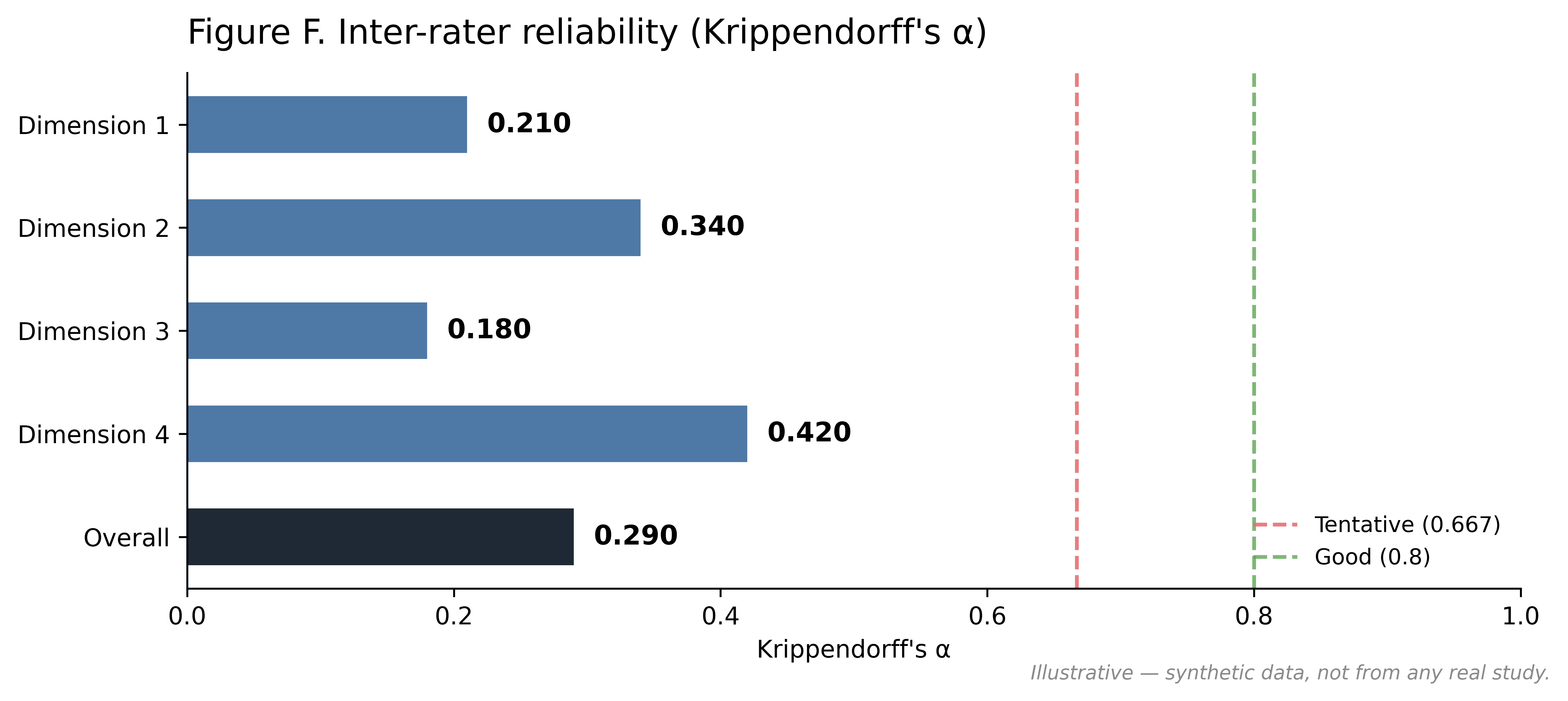
6.1 Krippendorff's α on scalar ratings
Krippendorff's α is a general-purpose coefficient of agreement that handles arbitrary numbers of raters, missing data, and multiple measurement levels (nominal, ordinal, interval). It returns a value in (−∞, 1], where 1.0 indicates perfect agreement, 0 indicates agreement at chance, and negative values indicate systematic disagreement.
Conventional thresholds for substantive use are α ≥ 0.8 (acceptable), 0.667 ≤ α < 0.8 (tentative, suitable for exploratory analysis only), and α < 0.667 (unreliable). α is computed on the scalar rating data with the interval distance function. α is consistently the lowest reliability number reported in any study, which is the expected pattern for absolute Likert ratings across heterogeneous human raters. Scalar means are reported with this caveat and treated as directional rather than absolute.
6.2 Krippendorff's α on rankings (ordinal)
α is recomputed on the rank data using the ordinal distance function, which penalizes large rank differences more heavily than small ones. Comparing the ordinal-rank α to the interval-scalar α quantifies how much agreement information is gained by switching from absolute rating to relative ranking. In practice rank α is meaningfully higher than scalar α, which is one of the reasons pairwise analyses receive primary weight in the report.
6.3 Kendall's coefficient of concordance (W) per flight
Krippendorff's α returns a single number for the entire study. Kendall's W returns a single number per flight: the proportion of variance in the panel's aggregate ranking that is explained by genuine consensus rather than noise. W ranges from 0 (no concordance) to 1 (perfect concordance), with W ≥ 0.5 conventionally interpreted as strong, 0.3 to 0.5 as moderate, and below 0.3 as weak. Per-flight W identifies which flights produced a clear consensus winner and which split the panel. The latter are flagged for closer inspection, since low concordance can indicate either that the bottlings are genuinely interchangeable on the flight in question or that the flight itself is ambiguous.
6.4 Pairwise Spearman rank correlation between evaluators
For every pair of evaluators, the Spearman rank correlation of their assigned ranks on the flights they both evaluated is computed. The full N-by-N correlation matrix is reported as a heatmap, and each evaluator is assigned a panel-fit score equal to the mean of their correlations with the rest of the panel. This diagnostic is primarily operational. It identifies a consensus cluster of evaluators whose judgments converge with the majority of the panel, and it flags outliers whose rankings diverge. Panel-fit scores feed directly into rehire decisions for future studies.
6.5 Hierarchical rater clustering
The pairwise Spearman correlations between evaluators are inverted into a distance matrix and passed through hierarchical agglomerative clustering. The resulting dendrogram is reported alongside the correlation heatmap and reveals whether the panel splits into stable subgroups (for example, a majority cluster of evaluators in broad agreement and a minority cluster with a different palate prior) or whether it behaves as a single population. Where multiple clusters exist, downstream analyses can be repeated within each cluster as a sensitivity check, and rubric calibration sessions for future studies can be designed to address the dimensions on which the clusters diverge.
6.6 Reporting
All five diagnostics are reported in every study rather than collapsed into a single number. A study with strong rank concordance and weak scalar agreement, for example, supports claims about ordering but not about absolute magnitude. A study with two clearly separated rater clusters supports claims within each cluster but warrants caution in aggregate. The reader is given the data needed to weight every quantitative finding accordingly.
7. Recruiting
7.1 Panel size
An Oenra Labs panel is typically composed of eight to twelve evaluators per study, with smaller pilot studies running as low as five and larger studies extending to fifteen. Panel size is chosen to balance two competing requirements: enough evaluators to produce stable aggregate rankings and to compute inter-rater reliability with meaningful confidence intervals (see §6), and few enough to allow thorough screening, onboarding, and per-study compensation at a sustainable cost.
7.2 Candidate profile
Evaluators are recruited from the Oenra taster network and, where domain expertise is specialized, from targeted outreach to partner wineries, importers and professional bodies. Every panelist for a study must satisfy a set of role-relevant criteria written specifically for the study's wine category. The general pattern is as follows.
- Active practitioner. The evaluator currently works in the target category as part of their day-to-day professional practice, not as a hobby or as a former practitioner.
- Mid-level or senior experience. Approximately four or more years of professional experience in the target category, sufficient to have internalized the judgment criteria the rubric is testing.
- Direct exposure to the category on trial. The evaluator has tasted wine of the kind being evaluated (for example, a study of aged Burgundy in the secondary market requires evaluators who regularly assess mature Pinot Noir in their own work).
- Demonstrated judgment on each rubric dimension. The evaluator can articulate what makes a bottling good or bad on every dimension of the study's rubric, validated during screening with a short calibration task.
- Comfortable with the workflow. The evaluator is willing and able to taste many side-by-side comparisons in sequence and to produce concise, useful written feedback.
The exact criteria are documented in a per-study participant brief that the recruiting team uses for outreach and screening.
7.3 Screening and onboarding
Candidates submit a brief résumé or tasting-history review during application. Recruiters check each candidate against the participant brief and run a short calibration exercise that mirrors the live study: a small number of representative flights, the same instrument the live study will use, and a debrief in which the candidate explains their rationale. Calibration notes are reviewed for rubric understanding rather than for "correct" answers; candidates who can articulate why they judged each pour the way they did are admitted to the panel.
Before live data collection begins, the admitted panel receives written guidelines that restate the rubric, define each scalar dimension, and walk through the evaluation interface. Time is left for clarifying questions in advance of the study window.
7.4 Compensation
Evaluators are paid a fixed honorarium per study. Honoraria are calibrated to the expected time commitment and to prevailing market rates for the evaluator's professional background, and typically fall in the low hundreds of US dollars for a one-week study window. Compensation is stated up-front in the participant brief and is not contingent on the direction of the evaluator's judgments.
7.5 Rehire criteria
Evaluator performance from completed studies is logged and used to inform invitations for subsequent studies. The principal performance signals are completion (did the evaluator finish their assigned tournaments inside the window), rationale quality (were the written responses specific, actionable, and grounded in the pours), and panel fit (how strongly did the evaluator's rankings correlate with the rest of the panel; see §6.4). Low panel fit is not in itself disqualifying. An outlier may be a domain specialist whose palate differs from the majority in a study-relevant way, but it is reviewed alongside the other signals when assembling future panels.